Dynamic Table in Snowflake : Implementing Type 2 Slowly Changing Dimensions (SCD) with Flexibility and Efficiency

Introduction:
Snowflake introduced ‘Dynamic Tables’ as a new feature in 2022. Dynamic tables can significantly simplify data engineering in Snowflake by providing a reliable, cost-effective, and automated way to transform data for consumption.
In this blog, we will discuss what a dynamic table is, when to use it and we’ll also build SCD type 2 using the dynamic table with an example.
Dynamic Table:
Dynamic tables are a new table type in Snowflake that lets teams use simple SQL statements to declaratively define the result of data pipelines. They also automatically refresh as the data changes, only operating on new changes since the last refresh. The scheduling and orchestration needed to achieve this are also transparently managed by Snowflake.
Comparison of materialised views with dynamic tables
Materialised view vs dynamic table:
Dynamic tables come with certain advantages, use cases and of course, challenges.
Advantages:
- Flexibility: Dynamic tables offer flexibility in that they can alter their structure or schema on the fly. Depending on particular circumstances or occurrences, columns may be added, modified, or eliminated.
- Data Structures: Dynamic tables can handle structured and unstructured data.
- Real Time Data: Dynamic tables can be updated in real-time as new data arrives, so the latest information is available immediately.
Disadvantages:
- Queries: Querying dynamic tables may require more complex and flexible query logic to handle the changing schema or structure of the data.
- Data Integrity: It can be more difficult to ensure data integrity and maintain consistency when dynamic tables’ schema can vary, especially when relational constraints are involved.
While materialised views have other strengths, weakness and use cases:
Advantages:
- Performance: Materialised views are pre-computed and stored copies of data that originate from one or more source tables. They are used to optimise query performance by reducing the need for expensive calculations or query-time joins.
Disadvantages:
- Fixed structure: Adding or removing columns in materialised views usually requires a rebuild of the view.
- Data Consistency: In order to guarantee data consistency with the source tables, materialised views are often refreshed on a frequent basis. The automatic maintenance of materialised views consumes credits.
Section 1: Preparing Your Data Structure
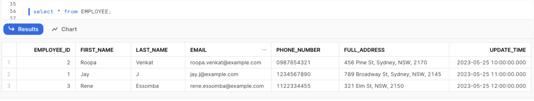
Create the EMPLOYEE Table and insert the sample data.
1
2
3
4
5
6
7
8
9
CREATE OR REPLACE TABLE EMPLOYEE (
  EMPLOYEE_ID INT,
  FIRST_NAME VARCHAR(50),
  LAST_NAME VARCHAR(50),
  EMAIL VARCHAR(100),
  PHONE_NUMBER VARCHAR(15),
  FULL_ADDRESS VARCHAR(365),
  UPDATE_TIME TIMESTAMP_NTZ(9)
);
1
2
3
4
5
6
INSERT INTO EMPLOYEE
VALUES
(2, 'Roopa', 'Venkat', 'roopa.venkat@example.com', '0987654321', '456 Pine St, Sydney, NSW, 2170', '2023-05-25 10:00:00'),
(1, 'Jay', 'J', 'jay.j@example.com', '1234567890', '789 Broadway St, Sydney, NSW, 2145', '2023-05-25 11:00:00'),
(3, 'Rene', 'Essomba', 'rene.essomba@example.com', '1122334455', '321 Elm St, NSW, 2150', '2023-05-25 12:00:00');
Section 2: Using SQL to Create Dynamic Tables
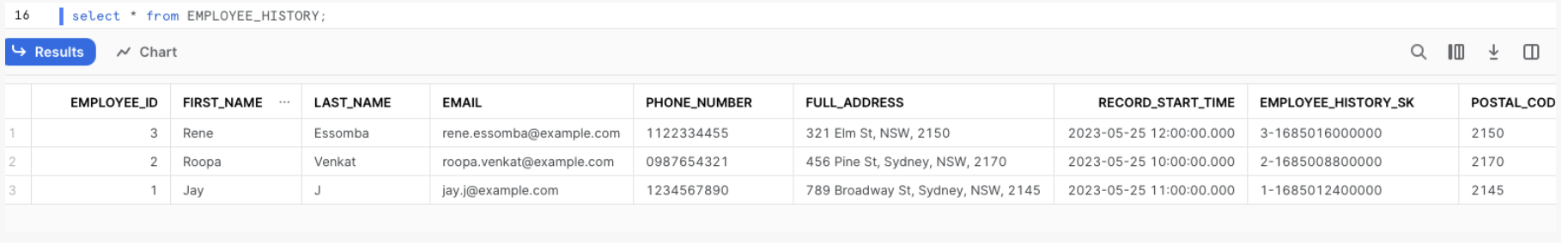
A dynamic table is created to track the time a record was active and to serve as a substitute key for a specific version of a customer’s data. A Type 2 SCD history table, this one. The surrogate key “EMPLOYEE_HISTORY_SK,” which is specific to each record in the table, can be used for historical analysis and to join data to a particular version of a customer’s information.
1
2
3
4
5
6
7
8
9
10
11
12
CREATE OR REPLACE DYNAMIC TABLE EMPLOYEE_HISTORY
TARGET_LAG='1 MINUTE'
WAREHOUSE=COMPUTE_WH
AS
SELECT * RENAME (UPDATE_TIME AS RECORD_START_TIME),
EMPLOYEE_ID || '-' || DATE_PART(EPOCH_MILLISECONDS, UPDATE_TIME) AS EMPLOYEE_HISTORY_SK,
SPLIT_PART(FULL_ADDRESS, ' ', -1) AS POSTAL_CODE,
CASE
    WHEN LEAD(UPDATE_TIME) OVER (PARTITION BY EMPLOYEE_ID ORDER BY UPDATE_TIME ASC) IS NULL THEN '9999-12-31 12:00:00' -- Replace with a valid NULL date representation in your database
    ELSE LEAD(UPDATE_TIME) OVER (PARTITION BY EMPLOYEE_ID ORDER BY UPDATE_TIME ASC)
  END AS LEAD_TIME
FROM EMPLOYEE;
A maximum lag of one minute is the aim set for the dynamic table. This ensures that data will never be delayed for longer than one minute, assuming proper warehouse provisioning.
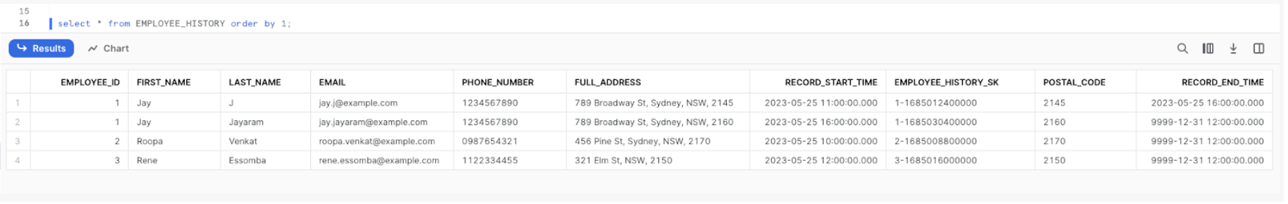
The current row’s update time is renamed as “RECORD_START_TIME” column, while the update time for the customer’s subsequent chronological row is listed in the “RECORD_END_TIME” column.
“RECORD_END_TIME” is set to max date, indicating that the record includes the most recent information about the client. The dynamic table can also be used to calculate any derived columns, such as “POSTAL_CODE” in this example.
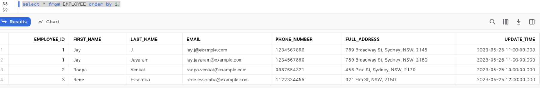
Section 3 : Update the source records and verify the dynamic table
1
2
3
INSERT INTO EMPLOYEE
VALUES
(1, 'Jay', 'Jayaram', 'jay.jayaram@example.com', '1234567890', '789 Broadway St, Sydney, NSW, 2160', '2023-05-25 15:00:00')
Source Result:
Target Result:
Streams and Tasks vs Dynamic Tables
Streams and tasks versus dynamic tables
With dynamic tables, data is received and altered from the base tables in response to a written query that specifies the desired outcome. The frequency of these refreshes is determined by an automatic refresh procedure, ensuring that the data satisfies the set freshness (lag) target. While joins, aggregations, window functions, and other SQL constructs are permissible in the SELECT statement for dynamic tables, calls to stored procedures, tasks, UDFs, or external functions are not permitted.
However, Streams and Tasks provide additional flexibility. You can use Python, Java, or Scala-written user-defined functions (UDFs), user-defined table functions (UDTFs), stored procedures, external functions, and Snowpark transformations.
Furthermore, streams and tasks offer flexibility in managing dependencies and scheduling, which makes them perfect for handling real-time data synchronisation, notifications, and task triggering with complete process control.
Check out my previous blog to see how Stream and Task can be implemented
Dynamic tables are best used when:
In certain circumstances, it could be required to process data where its structure needs to be flexible or doesn’t fit into a predetermined format. Dynamic tables come into play in this situation. Dynamic tables provide you more control over handling changing or unpredictable data structures.
Use cases for dynamic tables include the following:
Removes the need to manage data refreshes, track data dependencies, or write one’s own code. Reduces the complexity of stream and job. Doesn’t require precise control over the refresh schedule. Materialisation of the results of a query of multiple base tables. To summarise, materialised views are fantastic for improving the efficiency of repeated queries, but dynamic tables are perfect for building SQL-based data pipelines. A great option for tracking and controlling real-time data changes is streams and tasks.
Conclusion
In this post, we have discussed how to create the dynamic table and implement SCD Type 2 using it. With dynamic tables, managing SCDs becomes simpler and more efficient compared to traditional methods.
Note: This article was originally published on Cevo Australia’s website
If you enjoy the article, Please Subscribe.